
In fact the spin–spin potential (11.4) which we repeatedly used throughout this chapter is only a part of the chromomagnetic interaction
|
| (11.26) |
where S12 is the tensor operator. The tensor component V T plays a role for orbital momenta l > 0. In any potential model that includes only a vector-exchange piece V V and a scalar-exchange piece V S, the ratio of tensor to spin–spin is well defined. In the particular one-gluon model [103] for equal masses
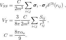 | (11.27) |
In Ref. [108] are listed the tests of chromomagnetism in baryon spectroscopy. Let us discuss here one example, the quadrupole deformation of Ω−.
The effect was first mentioned by Goldhaber and Sternheimer [109], who speculated on the fine and hyperfine structure of exotic atoms consisting of an atomic nucleus and an Ω−. The splitting pattern would provide a measurement of the quadrupole moment as well of the magnetic moment of the Ω−. In Ref. [109], a quadrupole moment Q = 1 fm2 was assumed for numerical illustration, on the grounds that the Ω− has a mass comparable to that of the deuteron and hence might also have Q of the same order of magnitude. In fact much smaller values of Q are obtained from current quark models [108, 110].
Let us adopt the same familiar notation 2S+1ℓ J as in quarkonium spectroscopy. The analogue of expansions (11.17) and (11.20) is [110]
 | (11.28) |
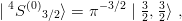
where n, p and q denote the successive hyperspherical harmonics of given spin and orbital momentum content. For an Ω− with spin S z = 3∕2, one needs only
 | (11.29) |
where the spin 3/2 wave function is given in Section 3.5, and
![√ ---[∘ --
4 (0) ---12- 2 2 2 3 1
| D 3∕2⟩ = π3∕2ξ2 5(ρ+ + λ+ ) | 2,− 2⟩
∘ --
− 45(ρ+ρ3 + λ+ λ3) | 32, 12⟩
∘ --- ]
+ 2(ρ23 + ρ+ ρ− + λ23 + λ+ λ− ) | 3, 3⟩ ,
15 2 2](baryon1489x.png) | (11.30) |
where ρ± = ∓(ρx ± ρy)∕ and ρ3 = ρz are the usual standard components of
  . Indeed, the
unperturbed wave function is dominated by its hyperscalar component and the quadrupole
operator
. Indeed, the
unperturbed wave function is dominated by its hyperscalar component and the quadrupole
operator
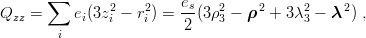 | (11.31) |
connects ∣4S(0) 3∕2⟩ only with ∣4D(0) 3∕2⟩. We end with equations very similar to those involved for the neutron charge radius
![e ∫∞
Q Ω = ⟨Qzz ⟩ = √-s-- u0 ξ2w0dξ ,
10
0 √ --
′′ 63-- C--96--2-u0(ξ)-
w 0 − 4ξ2w0 + ms [E0 − V0,0]w0 = ms π2√5-- ξ3 .](baryon1493x.png) | (11.32) |
Restricting the quadrupole deformation to a mixing of closest unperturbed states is exact for harmonic confinement, but leads us to underestimate QΩ by 20% for a smooth potential β = 0.1. The latter model, with the parameters (11.19), gives QΩ = 0.004 fm2.
Note that the dependence on the exponent β is rather simple, if one restricts oneself to
power-law potentials of the type (11.18). The strength of confinement, B, is determined from any
excitation energy, for instance the orbital splitting E ≡ E(2+) − E(0+), while the strength of
hyperfine corrections is measured by the mass shift ΔM =  of the ground state. One can
easily show [110] that QΩ scales as ΔM∕(E2m
s) (and, in turn, ΔM is related by scaling to
measurable mass shifts like Δ − N). In other words, choosing a confining potential fixes the
reduced quadrupole moment qΩ = QΩE2m
s∕ΔM, and qΩ varies by less than a factor of 2 when
going from a very smooth to a very sharp confinement. The phenomenological uncertainties come
mainly from the choice of strengths B and C, i.e., from different adjustments of excitation energies
and hyperfine splittings. The same scaling laws also hold for the charge radius of the
neutron.
of the ground state. One can
easily show [110] that QΩ scales as ΔM∕(E2m
s) (and, in turn, ΔM is related by scaling to
measurable mass shifts like Δ − N). In other words, choosing a confining potential fixes the
reduced quadrupole moment qΩ = QΩE2m
s∕ΔM, and qΩ varies by less than a factor of 2 when
going from a very smooth to a very sharp confinement. The phenomenological uncertainties come
mainly from the choice of strengths B and C, i.e., from different adjustments of excitation energies
and hyperfine splittings. The same scaling laws also hold for the charge radius of the
neutron.