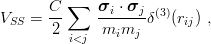
Systematics of hyperfine splittings

11.2 Systematics of hyperfine splittings

If one adopts a spin–spin potential analogous to the Breit–Fermi contact term in atomic physics, namely [103]

∑ V = C- σi ⋅-σjδ(3)(r ) , SS 2 mimj ij i<j

(11.4)

and treats it at first order, one achieves a good phenomenological description of hyperfine splittings. In the approximation of SU(3)_F flavour symmetry for the wave function, the correlation coefficients δ_ij ≡ ⟨ (3) ⟩
δ (rij) are the same for all pairs in any ground-state baryon of the SU(3)_F octet and decuplet, and one can derive amazing relations [103] such as

Ξ∗ − Ξ = Σ ∗ − Σ , ∗ 2Σ + Σ − 3Λ = 2(Δ − N ) .

(11.5)

Now, it is interesting to actually compute the correlation coefficients δ_ij and examine to what extent they depend on the quark i and j involved, and on the third quark.

To start with something simple, let us consider the ratio

2δ(Ω− ) δ (sss )( m )2 R3 = -------= -ss----- --q ⋅ Δ − N δqq(qqq ) ms

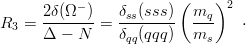(11.6)

that measures the ratio of the (non-observable) spin–spin shift δ(Ω⁻) of the Ω⁻ to the hyperfine splitting for ordinary baryons. Using the simple scaling laws (2.14), one gets

( ) mq- (1+2β)∕(r2+ β) R3 = m . s

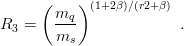(11.7)

For the small values β ≃ 0.1 mocking the combined effects of a Coulomb and a linear potential, the contraction of the wave function as m increases compensates a large part of the m⁻² dependence of the spin–spin operator.

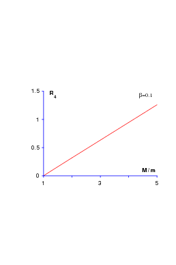
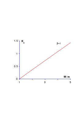
We now turn to more elaborate calculations where one has to account for the disymmetry of the wave function. First, we consider the Σ − Λ mass difference, a longstanding problem in baryon spectroscopy. The ratio

Σ--−-Λ- R4 = Σ ∗ − Σ

(11.8)

is experimentally R₄ ≃ 0.41. In the model (11.4), it is

δ12 − δ13(mq ∕ms) R4 = 2 ----------------- 3δ13(mq ∕ms )

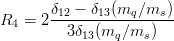(11.9)

and, as seen in Fig. 11.3, it is slightly lower than the experimental value R₄ ≃ 0.41, if one adopts standard values m_s < ∼ m_q for the constituent masses. Note that pionic loops might improve the situation [104].

Figure 11.3: Ratio R₄ = (Σ − Λ)∕(Σ^∗ − Σ) for the power-law potentials ∑ r_ij^β with β = 0.1 and β = 1, as a function of the quark mass ratio x = M∕m

On the other hand, the ratio

2 Σ∗ + Σ − 3Λ δ (qqs) R5 = -------------- = -qq----- , 2Δ − 2N δqq(qqq)

(11.10)

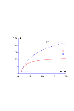
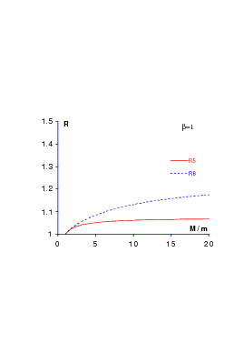
which focuses on the comparison of qq correlations in qqs and qqq systems, is reasonably well reproduced. For harmonic confinement, R₅ = 1 since the ρ and λ oscillators decouple exactly. As seen in Fig. 11.4, with a smooth potential r^β, β ≃ 0.1, one accounts for the experimental value R₅ = 1.04 [5], whose departure from 1 was noticed by Cohen and Lipkin [102]. Similarly, the ratio

Ξ∗ − Ξ δ (ssq) R6 = ------- = -sq----- Σ ∗ − Σ δsq(qqs )

(11.11)

turns out to be R₆ ≃ 1.16 experimentally, while a strict R₆ = 1 would be implied by SU(6) symmetry. In the harmonic oscillator, this ratio is close to 1 but not exactly equal to 1. With a smooth confinement, one gets a larger value, as seen in Fig. 11.4. Further evidence for the Cohen–Lipkin effect is shown in Ref. [105].

Figure 11.4: Ratios R₅ = (2Σ^∗ + Σ − 3Λ)∕(2Δ − 2N) and R₆ = (Ξ^∗− Ξ)∕(Σ^∗− Σ) for the power-law potentials ∑ r_ij^β with β = 0.1 and β = 1, as a function of the quark mass ratio M∕m

[next] [prev] [prev-tail] [front] [up]