
We first consider the case where the harmonic-oscillator Hamiltonian (3.43) is perturbed by a small additional potential
|
| (8.1) |
We note δ(n,l) the two-body matrix elements
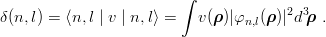 | (8.2) |
and notice that, thanks to the polynomial (times a Gaussian) structure of the h.o. wave functions, one can express all matrix elements in terms of the δ(0,l)’s which occur for nodeless states. For instance
 | (8.3) |
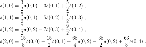
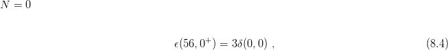
It is easy to compute the energy shifts due to δV in terms of these two-body matrix elements δ(n,l) and, in turn, to express the results with the δ(0,l) only. Of course, one has to make use of the permutation properties of the wave functions. One gets:

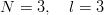
![− 3
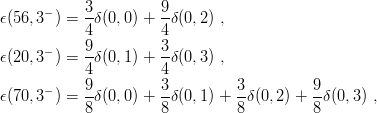
ϵ(70,1 ) = 2[δ(0,0) + δ (0, 1)]](baryon1278x.png) | (8.5) |
(the mixed symmetry partners remain degenerate to all orders),

 | (8.6) |
 | (8.7) |
 | (8.8) |
 | (8.9) |
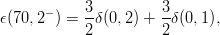
The perturbation mixes the ∣70, 1−⟩′ and ∣70, 1−⟩′′ states. One has to diagonalize the matrix
 | (8.10) |
![ϵ′ = 3-[19δ(0,0) + 13δ(0,1) − 35δ(0,2) + 35δ(0,3)]
32
′′ 1--
ϵ = 32[21δ(0,0) + 27δ(0,1) + 27δ(0,2) + 21δ(0,3)]
√ --
t = 3--5[− δ(0,0) + 9δ(0,1) − 15δ(0,2 ) + 7δ(0,3)].
32](baryon1288x.png) | (8.11) |
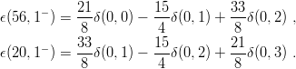
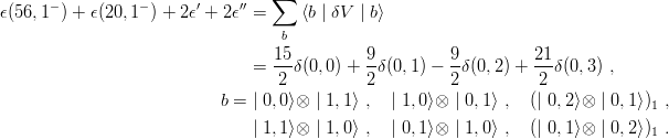
As a check, one can compute the trace of v in each (N,l) subspace using either the symmetrized basis ∣56,lP ⟩,∣20,lP ⟩, etc. or the original basis ∣n ρ,lρ⟩⊗∣nλ,lλ⟩. For instance, in the (N = 3, lP = 1−) case, one has to satisfy
 | (8.12) |
This allows one to detect a misprint for ϵ(56, 1−) in the review by Hey et al.[6], and to check that their original expression [75] is correct, with the correspondence a = 3δ(0, 0), b = 9 2δ(0, 1), c = 45 2 δ(0, 2), d = 315 8 δ(0, 3).
The pattern of Eq. (8.6) for the N = 2 level has been analysed by several authors [76, 77, 78, 79]. One can set
![15 9 15
¯ϵN=2 = --δ(0,0) + -δ(0,1 ) +---δ(0,2) ,
16 8 16
Δ = 15[2δ(0,1) − δ(0,0) − δ (0, 2)].
4](baryon1290x.png) | (8.13) |
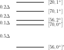
While the notation Δ = ϵ(20, 1+) − ϵ(56, 0+)′, corresponding to the overall spread of the N = 2 multiplet, has been adopted by all authors, the choice of N=2 seems rather arbitrary. The above prescription, as we shall see in Section 8.2, corresponds to the hyperscalar contribution of the perturbation δV . With (8.13), one can rewrite the N = 2 shifts (8.6) as
 | (8.14) |
corresponding to the famous splitting pattern of Fig. 8.1.
It has been noticed [37] that Δ is positive for any attractive power-law potential ϵ(α)rα, where ϵ is the sign function. In particular, if the popular
Coulomb-plus-linear potential is split into its best harmonic approximation (for N = 2) and a correction to it, say
 | (8.15) |
then one gets Δ > 0. In fact, the splitting parameter Δ measures the concavity of the leading Regge trajectory, for a nearly harmonic two-body potential. Thus from the perturbative version of the theorem (2.38), we obtain [80, 79]
![d [ 1dv ]
Y ≡ --- ---- <> 0 =⇒ Δ >< 0 .
dr rdr](baryon1294x.png) | (8.16) |
The appearance of this differential operator is not surprising, since Δ has to vanish if v(r) is constant or harmonic.
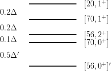
There are generalizations, where one has to give the collective radial excitation [56, 0+]′ a special treatment, whereas the separation between the four states [20, 1+], [70, 1+], [56, 2+] and [70, 0+] remains in the simple ratio 2:2:1, as illustrated in Fig. 8.2.
This occurs for a three-body perturbation of the harmonic oscillator [81], or as explained in the next Section, for nearly hyperscalar potentials.
The structure of the N = 3 multiplet was analysed by A.J.G. Hey et al.[6, 75] in terms of the rather powerful but abstract SP(12,C) group symmetry, and also by Cutkosky and Hendrick [38] and by Taxil et al.[79], who used more modest tools. If one defines
![3
¯ϵN=3 = 32-[7δ(0,0) + 9δ(0,1) + 9δ(0,2) + 7 δ(0,3)] ,
3
η = --{[2 δ(0,1) − δ (0,0 ) − δ(0,2)] + [2δ (0, 2) − δ(0,1) − δ(0,3)]} ,
8
γ = − 3-{[2 δ(0,1) − δ (0,0 ) − δ(0,2)] + [2δ (0, 2) − δ(0,1) − δ(0,3)]} ,
4](baryon1296x.png) | (8.17) |
one gets
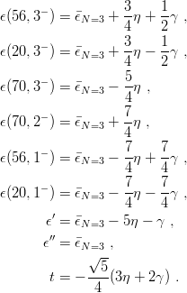 | (8.18) |
There is an overall shift N=3 of the levels and then all spacings are governed by the two quantities η and γ. This is illustrated in Fig. 8.3, for a linear perturbation to the harmonic oscillator.
One may rewrite the quantities η and γ as
![3
η = --[f (1 ) + f (2 )] ,
8
γ = 3-[f (2 ) − f (1 )] ,
4](baryon1298x.png) | (8.19) |
where again f(l) = 2δ(0,l) − δ(0,l − 1) − δ(0,l + 1) measures the concavity of the lowest Regge trajectory and is thus governed by the sign of Y
 | (8.20) |
The quantity γ is a kind of discretized third derivative in l. It was shown in Ref. [79] that
![[ ( ) ]
-d- 1-d- 1-dv- > <
W ≡ dr rdr r dr < 0 =⇒ γ > 0,](baryon1300x.png) | (8.21) |
provided that lim r→0r3v = 0. One can hardly guess the form of the differential operator W
without some preliminary study. In fact, if one introduces a perturbation v = Brβ, one gets by
straightforward calculation that γ ∝ Bβ(β − 2)(β − 4). It vanishes for β = 0 and β = 2, as
expected, and also for β = 4, leading to the expression of W![[v(r)]](baryon1301x.png) . The proof of (8.21) can be
sketched as follows. One starts from
. The proof of (8.21) can be
sketched as follows. One starts from
![∫∞ [ ]
γ = 3- v(r)dr (2u20,2 − u20,1 − u20,3) − (2u20,1 − u20,2 − u20,0) ,
4
0](baryon1302x.png) | (8.22) |
and performs a sequence of integrations by parts which transform the integral into
![∞∫
γ = 3- W [v(r)]K (r)dr
4
0](baryon1303x.png) | (8.23) |
From the explicit expression of the harmonic-oscillator radial functions un,l2(r), one gets K(r) ∝−r7 exp(−r2), which always remains negative. More details can be found in Ref. [79].