Let us come back to the reduced and rescaled Hamiltonian
|
| (3.43) |
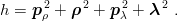
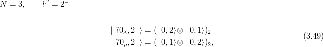
The wave functions are often labelled with N, the number of quanta, with lP , the total angular momentum and parity, and with the dimension of the SU(6) representation. The Hamiltonian (3.43) has, indeed, a symmetry of structure U(6) ≡ SU(6) × U(1), where U(1) is associated with the number of quanta N [6]. In fact, SU(6) also denotes another symmetry combining spin and flavour. It becomes exact when one neglects hyperfine effects and takes the limit of equal quark masses mu = md = ms. We refer to the specialized literature [6] for these group theoretical aspects of the harmonic oscillator. For our purpose, it is sufficient to know the following correspondence between SU(6) representations and permutation properties:
![[56] = symmetric
[20] = antisymmetric
[70] = mixed symmetry .](baryon1115x.png) | (3.44) |
By superposition of the factorized states (3.23), one can form:
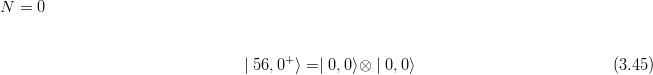
![N = 3, lP = 3−
1 √ --
| 56,3− ⟩ =-[| 0,0⟩⊗ | 0,3⟩ − 3(| 0,2⟩⊗ | 0,1⟩)3]
2 √--
| 20,3− ⟩ = 1[ 3 (| 0,1⟩⊗ | 0,2⟩)3− | 0,3⟩⊗ | 0,0⟩]
2 (3.48)
− 1-√--
| 70λ,3 ⟩ = 2[ 3 | 0,0⟩⊗ | 0,3 ⟩ + (| 0,2 ⟩⊗ | 0,1⟩)3]
1 √ --
| 70ρ,3− ⟩ =-[(| 0,1⟩⊗ | 0,2⟩)3 + 3 | 0,3⟩⊗ | 0,0⟩]
2](baryon1119x.png)
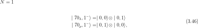
![N = 3, lP = 1−
1 √ -- √ --
| 56,1− ⟩ = √---[− 3 | 0,0⟩⊗ | 1,1⟩ + 5 | 1,0⟩⊗ | 0,1⟩ + 2(| 0,2⟩⊗ | 0,1⟩)1]
12
− --1-- √ -- √ --
| 20,1 ⟩ = √12--[− 3 | 1,1⟩⊗ | 0,0⟩ + 5 | 0,1⟩⊗ | 1,0⟩ + 2(| 0,1⟩⊗ | 0,2⟩)1]
1 √ -- √ --
| 70λ,1− ⟩′ =-√--[ 5 | 0, 0⟩⊗ | 1,1⟩ + 3 | 0,1⟩⊗ | 1,0⟩]
2 2
− ′ --1--√ -- √ -- (3.50)
| 70ρ,1 ⟩ = √--[ 5 | 1, 1⟩⊗ | 0,0⟩ + 3 | 0,1⟩⊗ | 1,0⟩]
2 2 √ -- √ --
| 70λ,1− ⟩′′ = √-1-[ 3 | 1, 1⟩⊗ | 0,0⟩ − 5 | 1,0⟩⊗ | 0,1⟩ + 4(| 0,2⟩⊗ | 0,1⟩)1]
24
− ′′ 1 √ -- √ --
| 70ρ,1 ⟩ = √----[ 3 | 1, 1⟩⊗ | 0,0⟩ − 5 | 0,1⟩⊗ | 1,0⟩ + 4(| 0,1⟩⊗ | 0,2⟩)1].
24](baryon1121x.png)
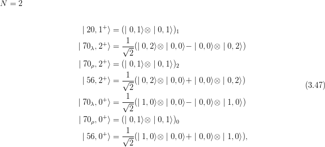
Up to N = 2 or even N = 3, one can obtain these combinations of the factorized states
∣nρ,lρ⟩⊗∣nλ,lλ⟩ by empirical methods. For instance, dealing with a scalar (l = 0) polynomial of
degree 2, one easily identify  2 +
2 +  2 as being symmetric, whereas
  2 −
2 − 2 and −2
 ⋅
⋅ form a pair
of mixed symmetry. For larger N, however, one hardly avoids the use of more systematic methods.
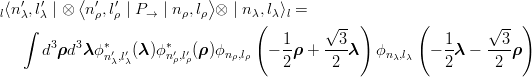
In each eigenspace labelled by N, with energy 6 + 2N, one can consider the subspaces (N,l) of
given total angular momentum and in each subspace diagonalize the permutation operator P→
(P12 is already diagonalized by the even or odd character of lρ). The relevant matrix
elements
form a pair
of mixed symmetry. For larger N, however, one hardly avoids the use of more systematic methods.
In each eigenspace labelled by N, with energy 6 + 2N, one can consider the subspaces (N,l) of
given total angular momentum and in each subspace diagonalize the permutation operator P→
(P12 is already diagonalized by the even or odd character of lρ). The relevant matrix
elements
 | (3.51) |
(the Clebsch–Gordan summations are omitted for better reading in the integral) are called the
Brody–Moshinsky coefficients [42]. They can be computed by astute recursion relations [43, 44], or (still exactly) by brute force computer algebra. Other methods have been proposed, for instance by Horgan [45], to construct the harmonic-oscillator wave functions of given angular momentum, parity and permutation properties.