
We now present some mathematical properties of two-body Hamiltonians. In one or two dimensions, any attractive potential supports at least one bound state (some local attraction is sufficient) [29]. In three dimensions, this is not true any more. For instance, a Yukawa potential V = −B exp(−αr)∕r, with α > 0, does not provide any bound state if B is too small. For α = 0, on the other hand, one gets the Coulomb potential, which has an infinite number of bound states, with E < 0, as well as a continuum spectrum of positive energies. In simple models of quarkonium, we are dealing with confining potentials, which support an infinite number of bound states.
From the Sturm–Liouville theorem [22] and the positivity of the centrifugal barrier l(l + 1)∕r2, the ground state always corresponds to n = 0 and l = 0 (the local character of V (r) is crucial here) and the energy increases with n or with l. The relative position of the radial and orbital excitations depends, however, on the shape of V (r). Figure 2.1 shows the location of the first levels for V = −1∕r, V = r, and V = r2.
The ordering and spacing patterns are rather different for these simple examples. For more general potentials, the following results have been obtained:
i) The
Coulomb theorem
If V (r) = −r−1, then E n,l = En+1,l−1. Remember that n denotes the number of nodes, not the principal quantum number of atomic physics, which is n + l + 1. The following theorem was proved, first for the lowest levels or for small perturbations around the Coulomb case, and later in a general way [30]
|
| (2.36) |
Note that one hardly elaborates a necessary condition on the potential for such a spectral property, since the binding energies do not uniquely determine the potential.
The Coulomb theorem ensures that the quarkonium potential V (r) = −a∕r + br gives the desired ordering Ψ′ > χ in charmonium and ϒ′ > χb in bb . The condition ΔV > 0 can be read as the charge seen by the quark increasing when the distance to the antiquark increases, in agreement with the ideas of asymptotic freedom and confinement. The theorem also has applications in atomic physics. If a low-lying muon μ− starts experiencing the size of a nucleus A, then one expects E1,0 > E0,1, or E2S > E2P in the usual notations, for the Aμ− system, as it is observed. On the other hand, for alkali atoms, i.e., for an external electron in the field of a nucleus surronded by close spherical shells of electrons, E1,0 < E0,1, again in agreement with observation.
ii) The
harmonic-oscillator theorem
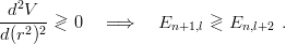
If V (r) = r2, then E n,l = En+1,l+2. This degeneracy is broken in the following way [30]:
 | (2.37) |
For instance, if one describes the charmonium spectrum with the Coulomb-plus-linear model, one obtains the right ordering Ψ′′(D-state) > Ψ′(S-state). The theorem (2.37) will be useful in the three-body case since the two-body systems factorize out in the limit of harmonic forces.
iii) Regge trajectory
In the harmonic-oscillator case, E0,l ∝ (3 + 2l) grows linearly in l. The following result has been established [31]:
![[ ]
d-- 1-dV- >
Y (r) ≡ dr r dr < 0 =⇒ E (0,l) concave (or convex ) in l.](baryon148x.png) | (2.38) |
iv) Spacing of radial excitations
In the harmonic-oscillator case, at fixed l, the energy En,l ∝ (3 + 4n + 2l) grows linearly in n. This means that Δ = 0, where Δ ≡ En+1,l + En−1,l − 2En,l. If one considers a potential V (r), one can restrict oneself to the l = 0 case, and, otherwise, incorporate the centrifugal barrier into V . The following results have been established. If V (r) = r2 + v(r) is nearly harmonic, i.e., if v(r) is treated to first order, then [32]
![[ ( ) ]
d-- -d- 1dv- > 3 >
Z (r) ≡ dr dr rdr < 0 and lri→m0 r v = 0 = ⇒ Δ < 0 .](baryon149x.png) | (2.39) |
Counter examples show that this result does not always hold beyond perturbation theory.