The potential in Eq. (8.1) is a special case of a more general class of
nearly hyperscalar potentials
|
| (8.24) |
or, if one gives up the two-body character,
 | (8.25) |
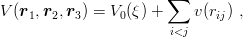
or equivalently, in the more abstract terms of the hyperspherical expansion of the potential
![V (r ,r ,r ) = π3∕2 [V (ξ)Q (Ω) + V (ξ)Q (Ω) + V (ξ)Q (Ω) + ...] ,
1 2 3 0 0 4 4 6 6](baryon1306x.png) | (8.26) |
where  0(Ω) = π−3∕2,
4(Ω), etc, are the lowest scalar and fully symmetric hyperspherical
harmonics, given in Section 5.2, and where the L > 0 components V 4, V 6,... are small. For
simplicity, we use the same notations α = [56, 0+], [70, 1−], [20, 1+]…as for the harmonic-oscillator
states to stress their angular momentum and permutation properties.
0(Ω) = π−3∕2,
4(Ω), etc, are the lowest scalar and fully symmetric hyperspherical
harmonics, given in Section 5.2, and where the L > 0 components V 4, V 6,... are small. For
simplicity, we use the same notations α = [56, 0+], [70, 1−], [20, 1+]…as for the harmonic-oscillator
states to stress their angular momentum and permutation properties.
If the potential V is nearly hyperscalar, one may approximate the wave function of each state by its lowest hyperspherical component, say
 | (8.27) |
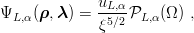
where uL,α and the binding energy are given by the single radial equation (m = ℏ = 1),
![′′ (L-+-3-∕2)(L-+-5∕2)
u L,α − ξ2 uL,α + [E − UL,α]uL,α = 0 ,](baryon1308x.png) | (8.28) |
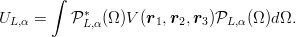 | (8.29) |
Inserting the expansion (8.26) results in the following expressions for the UL,α(ξ):

![+
[56, 0 ] V0(ξ) ,](baryon1311x.png) | (8.30) |

![[70, 1− ] V0(ξ) ,](baryon1313x.png) | (8.31) |

![√ --
[20,1+ ] V (ξ) + 5--3V (ξ) ,
0 1√5-- 4
3
[70,2+ ] V0(ξ) + ---V4(ξ) ,
1√5--
+ --3-
[56,2 ] V0(ξ) − 315 V4 (ξ) ,
√ --
[70,0+ ] V0(ξ) − 5--3V4 (ξ) ,
15](baryon1315x.png) | (8.32) |

![√ -- √ --
[56,3− ] V (ξ) + --3V (ξ) + --2V (ξ ) ,
0 √7--4 √7-- 6
3 2
[20,3− ] V0(ξ) + ---V4(ξ) − ---V6 (ξ ) ,
7√ -- 7
− 5--3-
[70,3 ] V0(ξ) − 21 V4(ξ) ,
√ --
[70,2− ] V0(ξ) + --3V4(ξ) ,
√3-- √ --
− 3 2
[56,1 ] V0(ξ) − -3-V4(ξ) + -2-V6 (ξ ) ,
√ -- √ --
[20,1− ] V (ξ) − --3V (ξ) − --2V (ξ ) ,
0 3 4 2 6
[70,1− ] V0(ξ) .](baryon1317x.png) | (8.33) |
These expressions can be obtained either by direct angular integration of Eq. (8.29), or by considering the special case V 0(ξ) = ξ2, and using the formula of Section 8.1 for the potentials v(rij) = rijn, with n = 0, 4 or 6. This enables us to switch on one after the other the L = 0, L = 4 and L = 6 multipoles of the potential. This is one more illustration of the many links between the hyperspherical formalism and the harmonic oscillator [43].
If one compares the Eqs. (8.32) with the N = 2 sequence in the harmonic oscillator as appearing in Eqs. (8.6) and (8.14), one notices the absence of the [56, 0+]. This state is a hyper-radial excitation of the L = 0 ground state. Similarly, the [70, 1−] state of the N = 3 band is a hyper-radial excitation of the L = 1 level.
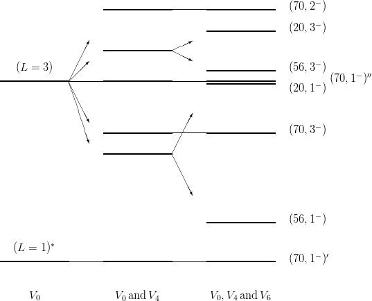
Now, if the radial equation (8.28) is first solved with V 0(ξ) alone and if the terms in V 4(ξ) and V 6(ξ) are treated at first order, one gets very simple relations between the energies. In the positive-parity sector, one gets the splitting pattern of Fig. 8.2. The negative-parity states are shown in Fig. 8.4. For illustration we have chosen a linear potential V = Σ rij, treated to first order around its hyperscalar approximation, but the ratios between the various splittings in each column are model-independent.