Numerical solution of the Faddeev equations

6.3 Numerical solution of the Faddeev equations

The set of coupled equations (6.8) can be solved numerically almost as it stands. For instance one can use the mapping and discretization procedure proposed in Section 2.4 for mesons. If r₀ is a plausible scale of the interquark distances, we introduce

ρ λ 1 x(ρ) = ρ-+-r- , y(λ ) = λ +-r- , ϕab(ρ,λ) = r-(1-−-x)(1-−-y)vab(x,y) , 0 0 0

(6.12)

∑ ∑N v (x, y) = v sin --iπn-- sin nπx sin jπm---sinn πy . ab abij N + 1 N + 1 i,j m,n=1

(6.13)

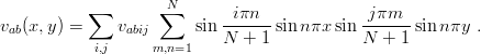
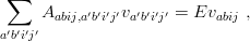
The v_abij, the unknowns of our problem, are the values of v_abij(x,y) at selected points [x_i,y_j] = [i∕(N + 1),j∕(N + 1)]. They are given, together with the energies E, by the matrix equation

∑ Aabij,a′b′i′j′va′b′i′j′ = Evabij , ′′′′ ab ij

(6.14)

ℏ2 Aabij,a′b′i′j′ = δaa′δbb′---2{t(xi,xi′)δjj′ + δii′t(yj,yj′)} mr 0 [ ] -ℏ2- (1 −-xi)2- (1-−-yj)2 + δaa′δbb′mr2 δii′δjj′ a(a + 1) x2 + b(b + 1) y2 0 i j + V[ρ(xi)][δaa′δbb′δii′δjj′ + (1 − xi)(1 − yj)Babij,a′b′i′j′] ,

(6.15)

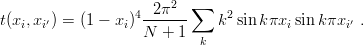
where the matrix elements of the radial kinetic energy have been already given in Section 2.4,

4--2π2- ∑ 2 t(xi,xi′) = (1 − xi) N + 1 k sin kπxi sinkπxi ′ . k

(6.16)

The most delicate (and time-consuming) part comes from the permutation operators. It reads

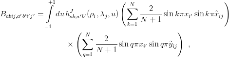+1 ( ) ∫ J ∑N 2 Babij,a′b′i′j′ = du hab;a′b′(ρi,λj,u ) ------sink πxi′ sin kπx˜ij −1 k=1 N + 1 ( N ) ∑ ---2-- × N + 1 sin qπxi′ sinqπ ˜yij , q=1

(6.17)

ρi = ρ(xi) λj = λ(yj) 1 ρ′ij = -(ρ2i + 3λ2j − 2ρiλju )1∕2 2 λ′ = 1(3ρ2 + λ2 + 2ρ λ u )1∕2 ij 2 i j i j ˜xij = x(ρ′ij) ′ y˜ij = y(λij) .

(6.18)

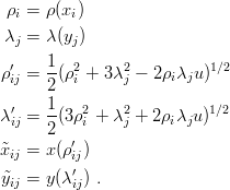
Among the many possible variants, one consists of using polar coordinates

ρ = r sin θ, λ = rcosθ ,

(6.19)

which are similar to the hyperspherical coordinates of Section 5.1. One can then perform the Fourier expansion in the rescaled variables x = r∕(r + r₀) and y = 2θ∕π. The advantage is that the kernel h conserves the hyper-radius r, thus reducing the number of times it has to be computed. If, however, the potential V (ρ) varies rapidly, one has to introduce many points in the discretization of the θ dependence, at least for large r.

[next] [prev] [prev-tail] [front] [up]