Solving the Faddeev equation

6.2 Solving the Faddeev equation

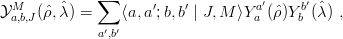
Since there are several ways of building a state of given total angular momentum J by combining the angular momenta l_ρ(≡ a) and l_λ(≡ b), let us introduce the normalized harmonics

M ˆ ∑ ′ ′ a′ b′ ˆ Y a,b,J(ˆρ,λ ) = ⟨a,a ;b,b | J,M ⟩Y a (ˆρ)Yb (λ ) , a′,b′

(6.6)

and the partial-wave expansion

∑ ϕ (ρ,λ) Ψ3 (ρ, λ) = -ab------YMa,b,J(ˆρ,ˆλ) . a,b ρλ

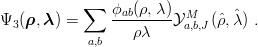(6.7)

The projection of the Noyes–Faddeev equation (6.5) gives

[ ] -1 -∂2- ∂2-- a(a +-1) b(b +-1) E + m ∂ρ2 + ∂λ2 − ρ2 − λ2 − V (ρ) ϕab(ρ, λ) ∫ +1 ∑ J (1) (1) = V (ρ) − 1 ha,b;a′,b′(ρ,λ,u)ϕa′b′(ρ ,λ )du . a′,b′

(6.8)

Here we notice that the P_→ and P_← terms give the same contribution. For computing the kernel h, we introduce the rotated coordinates ⁽¹⁾, ⁽¹⁾ and the angular variables u and u⁽¹⁾ given by

λ (1) + iρ(1) = j (λ + iρ ) , λ ⋅ ρ = λ ρu , λ (1) ⋅ ρ (1) = λ(1)ρ(1)u(1) ,

(6.9)

so that

∫ [ ]∗ ∫+1ρ(1)λ(1) d2ˆρ2d2ˆλ YMa,b,J(ˆρ,ˆλ) YMa′,b′,J (ρˆ(1),ˆλ(1)) = -------hJa,b;a′,b′(ρ,λ,u )du . ρ λ −1

(6.10)

Explicit expressions for h exist in the literature [64]. For the J = 0 case, h is simply given by

√-------√ ------ h0a,b;a′,b′ = --ρλ--- 2a + 1 2b + 1 δabδa′b′Pa(u)Pa ′(u(1)) , ρ(1)λ(1)

(6.11)

where P_n is a Legendre polynomial.

[next] [prev] [prev-tail] [front] [up]