There are hundreds of possible methods for solving the radial equation (2.5) for confining potentials, and many new suggestions can be found by reading journals of mathematical physics or computational physics as well as the American Journal of Physics and similar publications [24]. Let us describe briefly two methods: the Numerov method and the Multhopp method.
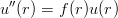
In the simplest of the direct numerical solutions of the radial equation (2.5), one separates the numerical integration in r at a given energy E, and the search for the eigenvalues. Hartree [25], for instance, gave an efficient method based on the Numerov algorithm, which nowadays can easily be implemented on computers or even on programmable calculators. Let us rewrite Eq. (2.5) as
|
| (2.18) |
and search for an outgoing uout(r) solution starting from uout(r) ∝ rl+1 near the origin and an
ingoing solution uin(r) starting from uin(r) ∝ exp(−∫
 dr) at large r. Using the Taylor
expansion and the above differential equation, one easily shows that the values un of uout (or of
uin) at equally spaced points r = nh fulfil
dr) at large r. Using the Taylor
expansion and the above differential equation, one easily shows that the values un of uout (or of
uin) at equally spaced points r = nh fulfil
 | (2.19) |
leading to a very accurate (and stable) iterative algorithm for computing the un’s.
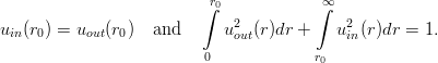
Now the (n + 1)th energy E n is determined as follows. A trial energy E is above En if the corresponding outgoing solution has at least (n + 1) nodes in ]0,rc[, where rc is the classical turning point, for which E = V (rc). One ends quickly with an interval an < En < bn in which En is the only possible eigenvalue. In this interval, En is the only value for which one can match the incoming and the outgoing solutions as well as their first derivative. One can always impose
 | (2.20) |
If u′in(r0) ⁄= u′out(r0) for some trial energy  , then a better estimate of En is given
by
, then a better estimate of En is given
by
![u(r0) ′ ′
^E − → ^E + dE^ = E^− --μ--[uin(r0) − u out(r0)]](baryon129x.png) | (2.21) |
Iterative applications of this recipe converge very rapidly towards En. Equation (2.21) may be
derived from the Wronskian theorem, whose many uses in quantum mechanics are well described in
Ref. [21]. Alternatively, one may consider that the mismatching solution {u(r) = uout for
0 < r < ro and u(r) = uin(r) for ro < r < ∞} corresponds exactly to the eigenvalue  for the
modified potential
for the
modified potential
 | (2.22) |
When first-order perturbation theory is applied to V starting from the solution of  , one gets
exactly the prescription (2.21).
, one gets
exactly the prescription (2.21).
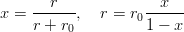
The application of matrix methods to quarkonium calculations was proposed independently by Basdevant et al.[26] and Olsson et al.[27] (and, probably, many others!). One of the many possible variants is the following. The transformation
 | (2.23) |
leads to the new equation
![1-(1 −-x)4 ′′ √ --
− μ r2 v (x) + V [r(x )]v(x) = Ev (x) , v(x) = (1 − x)u [r(x)] r0 ,
0](baryon134x.png) | (2.24) |
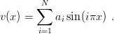
where v(x) is submitted to v(0) = v(1) = 0. The value of r0 should be chosen to be of the order of the typical radius of the wave function. One now computes v from its Fourier expansion
 | (2.25) |
For finite N, all information is contained in the ai’s and thus in the values vj of v(x) at the points xj = j∕(N + 1), since
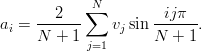 | (2.26) |
One ends with the matrix eigenvalue equation
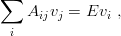 | (2.27) |
![( )
(1 − x )4 2π2 ∑N
Aij = -----2i-------- k2 sin kπxi sin kπxj + δijV [r(xi)] ,
μr0 N + 1 k=1](baryon138x.png) | (2.28) |
which is a matrix with
hidden symmetry. Indeed, the simple change of function
![--v(x)-- u[r(x)]√ --
w (x) = (1 − x)2 = 1 − x r0 ,](baryon139x.png) | (2.29) |
which, not surprisingly, corresponds to the simple normalization
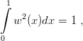 | (2.30) |
leads to the new matrix equation ∑ Bijwj = Ewi where, again, wj = w(j∕(N + 1)), and the matrix
![( )
(1 − xi)2(1 − xj)2 2π2 ∑N
Bij = ----------2------------- k2 sin kπxi sin kπxj + δijV [r(xi)]
μr 0 N + 1 k=1](baryon141x.png) | (2.31) |
is now symmetric. The diagonalization provides an approximation of the N first levels. A level of given radial number n is well described as soon as N ≫ n, and the convergence as N →∞ is reasonably achieved, provided the parameter r0 has been chosen to be of the right order of magnitude. The wave functions are mutually orthogonal, to the extent that the scalar product is replaced by its discretized approximation
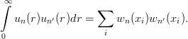 | (2.32) |
The tail of the wave function as r →∞ is, however, not too well reproduced, since the exponential vanishing of u(r) is replaced by a zero of finite order for w(x) at x = 1. The main advantage of this method, for our purpose, is its immediate generalization to coupled equations. This will be very useful for Faddeev, hyperspherical, or Born–Oppenheimer approaches to the three-body problem.
For illustration, we display in Table 2.1 the lowest eigenvalues of the linear potential V (r) = r in the case μ = 1, as a function of the dimension N of the matrix (2.31). The exact eigenvalues are given by the negative of the zeros of the Airy function [28]. The parameter r0 is chosen as being α0−1∕2 where exp(−α 0r2∕2) is the best variational approximation of Gaussian type to the ground state.
| (n,l) | N = 8 | N = 16 | N = 32 | Exact |
| (0, 0) | 2.33727 | 2.33810 | 2.33811 | 2.33811 |
| (1, 0) | 4.10306 | 4.08848 | 4.08795 | 4.08795 |
| (2, 0) | 5.25794 | 5.50337 | 5.52057 | 5.52056 |
| (0, 1) | 3.34873 | 3.36120 | 3.36125 | 3.36125 |
| (1, 1) | 5.03186 | 4.88522 | 4.88445 | 4.88445 |
| (0, 2) | 4.21405 | 4.24820 | 4.24818 | 4.24818 |