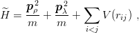
We consider here baryons qqQ with single flavour or QQq with double flavour. The quark masses are m1 = m2 = m and m3 = m′. The generalization to m1≠m2 is obvious. We use the Jacobi coordinates of Eq. (3.54) to deal with a unique reduced mass m. The reduced Hamiltonian,
|
| (4.12) |
looks formally the same as previously, but it is not symmetric under all permutations and it
contains some mass dependence hidden in λ. We still expand the solution of  into the eigenstates
of the symmetric h.o. The expansion mixes symmetric and mixed-symmetry states of the
h.o. basis. In the lP = 0+ sector, for instance, one should include 22 states if the h.o.
expansion is pushed up to N = 8: the 11 symmetric states listed in Eq. (4.3.4) and 11
mixed-symmetry states which are even under P12, the permutation of the first two
quarks.
into the eigenstates
of the symmetric h.o. The expansion mixes symmetric and mixed-symmetry states of the
h.o. basis. In the lP = 0+ sector, for instance, one should include 22 states if the h.o.
expansion is pushed up to N = 8: the 11 symmetric states listed in Eq. (4.3.4) and 11
mixed-symmetry states which are even under P12, the permutation of the first two
quarks.
For the numerical illustration, let us consider again a linear potential 1 2 ∑ rij and the sets of constituent masses (1, 1, 5) and (1, 1, 0.2) which are relevant for qqc and ccq charmed baryons, respectively. We display in Table 4.3 the behaviour of the ground state energy as a function of the maximal number of quanta, N, introduced in the expansion. Also shown is the order N′ to which the oscillator parameter K has been optimized. Some remarks are in order.
i) For small N, the convergence is slower than in the symmetric case. However, as soon as some basic mixed-symmetry components are included in the wave function, i.e., for N > 2, the convergence becomes much better.
ii) One may wonder why one chooses to expand an asymmetric system such as qqQ or QQq in terms of the symmetric h.o. hamiltonian H0. This does not favour the convergence and, as we shall see in the next section, alternative parametrizations of the trial wave function can be more efficient if the mass ratio m′∕m is very large or very small. The main advantage of the h.o. expansion is to allow for systematic computations of all matrix elements of interest. Those of V (r12) are simply
 | (4.13) |
For computing the matrix elements of V (r13), one has to perform the rotation
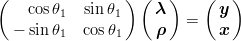 | (4.14) |
such that
 | (4.15) |
The matrix elements of V (rij) are immediate in the rotated basis ∣nx,lx; ny,ly⟩. To rewrite them in the original basis, one simply needs the Brody–Moshinsky matrix
 | (4.16) |
for which powerful recursion relations exist and computer codes are available [42, 43, 44].
| state | N | N′ | E0 |
| 0 | 0 | 3.4729 | |
| 2 | 0 | 3.4472 | |
| qqQ | 4 | 4 | 3.4390 |
| 6 | 4 | 3.4383 | |
| 8 | 4 | 3.4380 | |
| 0 | 0 | 5.0456 | |
| 2 | 0 | 4.9634 | |
| QQq | 4 | 4 | 4.9428 |
| 6 | 4 | 4.9403 | |
| 8 | 4 | 4.9395 | |