4.3 Harmonic-oscillator expansion (equal masses)
The method, which can also be used for mesons, is the following. One expands the eigenstates
of
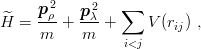 | (4.8) |
into the eigenstates of
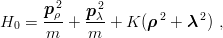 | (4.9) |
i.e.,
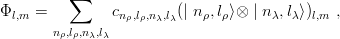 | (4.10) |
and studies the convergence as a function of the value of the maximal number of quanta allowed in
the expansion, N = 2nρ + lρ + 2nλ + lλ. In principle, one could optimize the variational parameter
K for each N. For high N, this results into expensive calculations and numerical instabilities. So,
in practice, one optimizes K for a small number of quanta N′ and then pushes the expansion up to
larger N. For given N and K, the harmonic-oscillator (h.o.) expansion results in the
diagonalization of a symmetric matrix, which is the restriction of  to the sub-space spanned by
the first levels of H0.
to the sub-space spanned by
the first levels of H0.
As an illustration, let us compute the two first levels having angular momentum and parity
lP = 0+, corresponding to quark masses m
i = 1 and a linear confinement. The h.o.
basis is made of these states with the label [56, 0+] in Section 3.6. We rename them
as
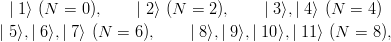 | (4.11) |
The results shown in Table 4.1 correspond to different prescriptions for the variational parameter
K, namely different levels of expansion N′ at which it is adjusted.
Table 4.1: Symmetric and scalar states ([56,0+]) for quark masses m
i = 1 and linear
confinement V = 1
2 ∑
rij using a harmonic-oscillator expansion up to N quanta. The
oscillator parameter K is adjusted by minimizing either the first or second level with an
expansion limited to N′ quanta (the minimized energy is underlined). The exact values are
very close to: E0,0 = 3.8631, E1,0 = 5.3207, and E2,0 = 6.5953.
|
|
|
|
|
|
| N | N′ | α = K1∕2 | E
0,0 | E1,0 | E2,0 |
|
|
|
|
|
|
| 0 | | | 3.8711 | | |
| 2 | | | 3.8711 | 5.3766 | |
| 4 | 0 | 0.4301 | 3.8640 | 5.3468 | 6.8082 |
| 6 | | | 3.8635 | 5.3214 | 6.6831 |
| 8 | | | 3.8632 | 5.3215 | 6.6008 |
|
|
|
|
|
|
| 4 | | | 3.8636 | 5.3695 | 7.0149 |
| 6 | 4 | 0.4782 | 3.8634 | 5.3259 | 6.7671 |
| 8 | | | 3.8632 | 5.3224 | 6.6364 |
|
|
|
|
|
|
| 2 | 0.3811 | | 3.8732 | | 3.8651 |
| 3.8639 | | 3.8634 |
| |
| | 5.3445 |
| 5.3388 | | 5.3223 |
| 5.3217 | |
| |
|
|
|
|
|
|
| |
As pointed out by Moshinsky [49], minimizing the ground state at the N′ = 2 order does not
provide any improvement with respect to N′ = 0. Otherwise, the value of the harmonic
oscillator parameter K depends rather sensitively on which level and to which order the
minimization is performed. However, the accuracy of the eventual energies depends less on
the prescription adopted for K than on the number of quanta N introduced in the
expansion.
Another output of such a calculation is the set of coefficients ci which describe the wave
function. For instance, in the case where K is optimized at the N′ = 4 order and the expansion
pushed up to N = 8, one obtains, for the wave function Ψ = ∑
ci∣ i⟩ of the ground state and its first
radial excitation the coefficients given in Table 4.2.
Table 4.2: Coefficients of the harmonic-oscillator expansion for the ground state and first
excitation with lP = 0+. It includes up to N = 8 quanta, but the oscillator strength is
determined by minimizing the ground state energy when the expansion is truncated at the
N′ = 4 level. Quark masses are mi = 1, and the interquark potential 1
2 ∑
rij.
|
|
|
|
|
|
| State | | | | | |
|
|
|
|
|
|
| n = 0 | 0.99431 | –0.08993 | | | –0.00494 | | –0.00232 |
| –0.00223 | |
| | 0.00115 | | –0.00178 |
| –0.00304 | | 0.00554 |
| |
|
|
|
|
|
|
|
| n = 1 | 0.10169 | 0.94301 | | | | –0.00454 | | 0.00486 |
| 0.00577 | | –0.02859 |
| |
|
|
|
|
|
|
|
| |
Note that the convergence is rather clear for the ground state, which is dominated by the
N = 0 component c1 ∣ 1⟩. There is more mixing of configurations for the excited states, as is usual in
variational calculations.