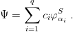
![[ ] 1
un,l(r) ∑q Γ (32 ) 2 √ --- l( αi) 34 1 2
Rn,l = --r----= ci ---3---- ( αir) π-- exp − 2αir ,
i=1 Γ (2 + l)](baryon1168x.png)
As already acknowledged, the h.o. expansion (as well as the hyperspherical expansion of Chapter 5) suffers from being a little heavy, especially in the case of unequal masses. Its main advantage is that convergence can eventually be reached, provided one pushes the calculation far enough. Now, there exist many alternative parametrizations of the trial wave function which immediately provide a dramatic accuracy, though they are a little empirical in nature. We shall present below the example of the parametrization of the wave function in terms of Gaussian functions. This method is copiously used in theoretical molecular physics.
Let us introduce the method in the simple two-body case. The radial wave function is written
|
| (4.17) |
and the αi’s and the ci’s are optimized, the latter being subject to a normalization constraint. For given αi’s, the ci’s are obtained by a simple matrix diagonalization. The αi’s are determined by standard minimization algorithms. The choice of the above parametrization leads to easy calculation of the matrix elements, most often in terms of elementary functions. With only the q = 1 term, the method coincides with the N = 0 order of the h.o. expansion. The comparison for increasing q and N is shown in Table 4.4, for angular momentum l = 0, reduced mass μ = 1, and potential V (r) = r. The Gaussian expansion is clearly more efficient here.
| Harmonic oscillator | Gaussian | |||
| 1 | N = 0 2.34478 | q = 1 2.34478 | |||
| 2 | N = 2 2.34478(1) | q = 2 2.33825 | |||
| 3 | N = 4 2.33841 | q = 3 2.33811 | |||
(1)The Moshinsky theorem [49] strikes again.
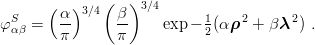
Consider now the case of symmetric baryons (qqq). The starting point coincides with the N = 0 order of the h.o. expansion
![S ( α)3 ∕2 [ 1 2 2 ]
Ψ = φα = π exp − 2α (ρ + λ ) .](baryon1169x.png) | (4.18) |
We name it
1S for
1 Gaussian with lρ = lλ = 0. We similarly define
2S,
3S,…parametrizations by superposing q = 2, 3…of these Gaussians.
 | (4.19) |
Incursions into the lρ = lλ > 0 sectors provide configurations
qP,
qD which can be added to the
qS ones. This makes use of
![P -2-- S
φ α(ρ, λ) = √3-α ρ ⋅ λ φα (ρ, λ)
[ ]
φDα(ρ, λ) = -√2--α2 3(ρ ⋅ λ )2 − ρ2λ2 φSα (ρ,λ), etc.
3 5](baryon1171x.png) | (4.20) |
For the qqq ground state with quarks of mass m = 1 bound by V = 1 2 ∑ rij, one obtains the results of Table 4.5.This is comparable to a harmonic-oscillator expansion pushed up to N = 6.
Consider now the cases of qqQ and QQq baryons, with constituent masses (1, 1, 5) and (1, 1, 0.2), respectively, and the same V = 1 2 ∑ rij. The terms of the variational wave function can now have different Gaussian parameters for the ρ and λ parts. For instance
 | (4.21) |
The results are shown in Table 4.5. With only one term, one already obtains a good approximation because the trial wave function can adjust itself to the asymmetry of the system. Note that, for QQq, internal orbital excitations play a less important role than the detailed description of the S-wave sector.
| Parametrization | qqq | qqQ | QQq |
| 1S | 3.8711 | 3.4451 | 4.9498 |
| 2S | 3.8648 | 3.4394 | 4.9414 |
| 3S | 3.8647 | 3.4391 | 4.9400 |
| 1S+1D | 3.8698 | 3.4441 | 4.9422 |
| 2S+1D | 3.8634 | 3.4383 | 4.9408 |