Introduction

4.1 Introduction

Variational calculations of few-body bound states have been designed and performed since the beginning of quantum mechanics. More and more elaborate methods have been used [46], in particular for atomic and molecular physics, where a high accuracy is often needed.

Since baryons present themselves as rather compact objects, with quarks tightly bound together, we do not need the ultimate refinements of variational techniques for computing their energy and wave functions. We shall thus restrict ourselves in this chapter to a simple introduction to elementary variational calculations. In fact, if one likes challenging few-body calculations, one should consider multiquark spectroscopy. A state such as qqq q

hesitates between a compact configuration, with all quarks close together, and a separation into qq + qq . A good variational wave function should incorporate these two components and this results in lengthy calculations [47].

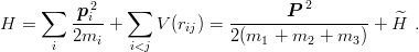
Coming back to baryons, we shall consider a Hamiltonian

∑ p 2i ∑ P 2 H = ----+ V (rij) = ----------------- + H^ . i 2mi i<j 2(m1 + m2 + m3 )

(4.1)

The extension to include spin–spin forces, or a flavour-dependent potential V _ij(r_ij), or three-body forces, does not lead to essentially new difficulties.

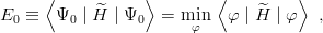
For the ground state, variational calculations are based on the Rayleigh–Ritz principle

⟨ ⟩ ⟨ ⟩ E0 ≡ Ψ0 | ^H | Ψ0 = min φ |H^ | φ , φ

(4.2)

and its consequence that if φ₀ = Ψ₀ + δΨ₀ is an approximation of the true wave function Ψ₀, the approximate energy ₀ = ⟨ ⟩
φ0 |H^ | φ0 departs from E₀ to second order only. In other words, the binding energy is always better approximated than the wave function, a property that one should keep in mind for the applications. The same minimization procedure can be applied to every ground state in a sector of some definite parity, angular momentum or permutation properties. Its energy can be approximated from above by using trial wave functions carrying appropriate quantum numbers.

The serious difficulties occur for radial excitations. One may ignore orthogonality problems and search for a stationary value of the functional

⟨ ⟩ E [φ] = φ |H^ | φ ,

(4.3)

for each level independently, but without any guarantee of success. A more systematic search consists of introducing a set of n orthogonal wave functions f_i(α; ,), spanning a sub-space _n(α), where α denotes all the parameters. For any given α, one diagonalizes the restriction of the Hamiltonian to _n(α), resulting in eigenvalues ϵ₀(α), ϵ₁(α)…ϵ_n−1(α). The best approximation to the j^th state consists of minimizing ϵ_j−1(α) with respect to α. In general, this leads to a different set of parameters α for each level, and orthogonality is lost. To restore orthogonality, one should adopt a compromise by fixing α at once for all levels of interest.

[next] [front] [up]