7.2 The Born–Oppenheimer approximation
The Born–Oppenheimer method is very often used in molecular physics and other few-body
problems and always turns out to be very efficient and to actually work better than expected. This
method seems particularly suited for baryons bearing two units of heavy flavour, since the heavy
quarks move much more slowly than the light quark.
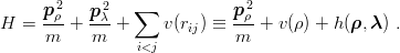
Let us consider a (1, 2, 3) = (QQq) baryon, with quark masses m, m and m′. The
generalization to m1≠m2 is obvious. With the Jacobi coordinates of Eq. (3.54), the Hamiltonian
reads
 | (7.3) |
By including the recoil of the charmed core, we greatly improve the accuracy of the calculation,
at no expense. For any fixed  , one can compute the eigenstates corresponding to the stationary
states of the light quark, i.e.,
, one can compute the eigenstates corresponding to the stationary
states of the light quark, i.e.,
 | (7.4) |
This corresponds to a one-particle problem in a non-central potential. Astute calculations could
make use of elliptic or bi-polar coordinates. In fact, one may simply use an ordinary expansion into
partial waves
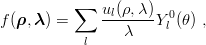 | (7.5) |
resulting in coupled equations for the ul’s.
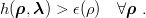
Consider first the ground state. If one adds the light-quark energy ϵ(ρ) to the direct
interaction between the heavy quarks, one gets the simplest (and well-known) form of the
Born–Oppenheimer approximation, sometimes referred to as the “extreme adiabatic”
[72]
![[ Δ ]
− --ρ+ v12(ρ ) + ϵ(ρ) ϕ0(ρ) = EEA ϕ0(ρ ) ,
m](baryon1252x.png) | (7.6) |
which overestimates the binding, i.e., is antivariational. Indeed, EEA ≤ Eexact results from the
operator inequality [33]
 | (7.7) |
The method is in fact more systematic. The exact wave function Ψ( ,
, ) of the (QQq) system
can be expanded as
) of the (QQq) system
can be expanded as
 | (7.8) |
reducing the three-body problem to an infinite set of coupled equations for the ϕn( ). Keeping
only the first term in the above expansion corresponds to a variational approximation, with a trial
wave function ϕ0f0. This is sometimes called [72] the
). Keeping
only the first term in the above expansion corresponds to a variational approximation, with a trial
wave function ϕ0f0. This is sometimes called [72] the
uncoupled adiabatic or
variational adiabatic approximation
![[ Δ ρ ⟨ Δ ρ ⟩ ]
− --- + v12(ρ) + ϵ(ρ) − f0 |--- | f0 ϕ0(ρ ) = EUA ϕ0(ρ) .
m m](baryon1258x.png) | (7.9) |
For improved calculations, one has to keep more terms in Eq. (7.8). An optimal choice
consists of grouping together the fn( ,
, ) in a combination which provides the maximal
correction. This is reminiscent of the potential harmonics in hyperspherical expansions, as
studied in Section 5.4. Here, we remark that f0(
) in a combination which provides the maximal
correction. This is reminiscent of the potential harmonics in hyperspherical expansions, as
studied in Section 5.4. Here, we remark that f0( ,
, ) is coupled to the higher adiabatics
through the kinetic energy. So, we use a normalized ∇
) is coupled to the higher adiabatics
through the kinetic energy. So, we use a normalized ∇ f0(
f0( ,
, ) to supplement f0(
 ,
, ),
namely
),
namely
 | (7.10) |
 | (7.11) |
Solving the two coupled equations in f0 and fb gives the so-called “coupled adiabatic”
approximation [72], which is always extremely close to (above) the exact result.
Detailed numerical studies of the Born–Oppenheimer approximation have been performed in
the context of studies of baryons with double charm [7, 73]. The method works quite well for ccq
configurations, as expected, but also for the ssq or even qqq cases. In Table 7.1, we display a
comparison of the extreme and uncoupled adiabatic approximations with exact results for the
mmm′ system with masses m = 1 and m′ = 0.2, 0.5 and 1, bound by the smooth 1∕2 ∑
rij0.1
potential. The quality of the approximation is impressive for both the energy of the first levels and
the short-range correlation.
What about the excited states in the Born–Oppenheimer approximation? We consider here the
optimal case m′≫ m. This implies that it is much more economical to excite the relative motion
of the heavy quarks than the motion of the light quark around them. For instance, in the harmonic
oscillator model, there is a ratio exactly [2m∕(2m′ + m)]1∕2 between the corresponding excitation
energies. Then, for the first excited states, the light-quark wave function remains in the lowest
adiabatic f0( ,
, ): the binding energy and the qq distribution is obtained from the low-lying
excited states of Eq. (7.9) or (7.6).
): the binding energy and the qq distribution is obtained from the low-lying
excited states of Eq. (7.9) or (7.6).
Higher states may also consist of an excitation of the light quark, corresponding to a dominant
 0fn component. In general, one hardly avoids mixing between such a configuration and
the previous ones, so that accurate estimates require solving coupled equations. Still,
the Born–Oppenheimer method provides one of the most efficient accesses to these
states.
0fn component. In general, one hardly avoids mixing between such a configuration and
the previous ones, so that accurate estimates require solving coupled equations. Still,
the Born–Oppenheimer method provides one of the most efficient accesses to these
states.
Table 7.1: Lowest levels and short-range qq correlations for qqq′ in the potential V =
1_
2 ∑
rij0.1, calculated either exactly or with two versions of the Born–Oppenheimer method,
the extreme and the variational adiabatic approximations
|
|
|
|
|
|
|
|
| m | m′ | Method | E0,0 | 103δ
12n=0 | E
1,0 | 103δ
12n=1 | E
0,1 |
|
|
|
|
|
|
|
|
| 1 | 0.2 | | | | | | |
|
|
|
|
|
|
|
|
| 1 | 0.5 | | | | | | |
|
|
|
|
|
|
|
|
| 1 | 1 | | | | | | |
|
|
|
|
|
|
|
|
| |