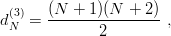
![--- ---
P 2 1 1∘ K 1 ∘ K
H = ----+ -KR 2 = -- ---h3 = -- ---[− Δ + r 2] ,
2M 2 2 M 2 M](baryon163x.png)
In the chapter on mesons, we already mentioned that the three-dimensional oscillator is solvable and may serve as a convenient basis for other potentials. The scale-independent part h3 of the Hamiltonian
|
| (3.6) |
can be written
 | (3.7) |
resulting in eigenvalues
 | (3.8) |
with eigenspaces of dimension
 | (3.9) |
which have a possible basis
 | (3.10) |
An alternative approach consists of using spherical coordinates, as in Section 2.1. This provides a new labelling of the eigenvalues
 | (3.11) |
Here l is the orbital momentum and n is the number of nodes of the reduced radial wave function un,l(r), whose expression is
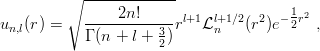 | (3.12) |
where  is a Laguerre polynomial
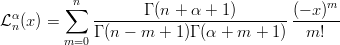 | (3.13) |
whose generating function is
 | (3.14) |
One may notice the useful relations
![[ ] √ -------
-d-− l +-1-+ r un+1,l(r ) = − 4n + 4 un,l+1(r) ,
dr r
[ d l + 1 ] √ -------
− ---− -----+ r un,l+1 (r ) = − 4n + 4 un+1,l(r) ,
[ dr r ]
-d- l +-1 √ -----------
dr − r − r un,l (r ) = − 4n + 4l + 6un,l+1(r) ,
[ ]
− -d-− l +-1-− r u (r ) = − √4n-+-4l-+-6u (r) ,
dr r n,l+1 n,l+1](baryon172x.png) | (3.15) |
and the useful integral
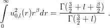 | (3.16) |
We have here a first example where levels are described in two different bases, namely ∣nx,ny,nz⟩ or ∣n,l,m⟩, with the restriction N = nx + ny + nz = 2n + l.